Segmentation#
In this Lab, we’ll be diving deeper into practical implementations of segmentation techniques, building on the concepts you’ve learned in the lecture.
What is Image Segmentation?#
Image segmentation is a crucial task in medical image analysis. It involves partitioning an image into multiple segments or regions, each corresponding to a different anatomical structure or area of interest. Accurate segmentation is essential for various medical applications, including:
Tumor detection and measurement
Organ volume estimation
Surgical planning
The idea of segmentation is that we classify each pixel as to whether it belongs to the region of interest or not. In the examples above the regions or interests are tumours, organs etc.
The Sliding Window Approach#
Before we dive into more advanced techniques, let’s briefly recap the sliding window approach, which has been a traditional method for image segmentation:
A fixed-size window “slides” across the image
For each window position, a classifier predicts whether the central pixel belongs to the target segment
This process is repeated for the entire image
While simple to implement, the sliding window method has some limitations: - It can be computationally expensive for large images - It doesn’t consider the full context of the image - The fixed window size may not be optimal for all structures
In this lab we will not be using the sliding window approach but instead we will be using a more advanced technique called the UNET.
[ ]:
# Some imports

import monai
import torch
from torch.utils.data import DataLoader
from monai.transforms import (
    EnsureChannelFirstd,
    AsDiscreted,
    Compose,
    LoadImaged,
    Orientationd,
    Randomizable,
    Resized,
    ScaleIntensityd,
    Spacingd,
    EnsureTyped,
    Lambda
)
import os
import tempfile
from utils.decathlon_dataset import get_decathlon_dataloader
from utils.unet import UNET
from utils.train import train

import matplotlib.pyplot as plt
MONAI Data Loading and Preprocessing for Hippocampus Segmentation#
The code in utils/decathlon_dataset.py demonstrates how to set up a data loading and preprocessing pipeline for the Hippocampus segmentation task using the MONAI library.
Directory Setup:
Establishes a root directory for data storage, either from an environment variable or a temporary directory.
Transform Pipeline:
Utilizes MONAI’s
Composeto create a sequence of transformations:LoadImaged: Loads image and label data.EnsureChannelFirstd: Ensures data has a channel dimension.Orientationd: Orients data to RAS (Right, Anterior, Superior) format.Spacingd: Resamples data to 1.0mm isotropic voxels.ScaleIntensityd: Scales image intensities.Resized: Resizes images and labels to 32x64x32 voxels.EnsureTyped: Ensures consistent data types.
Dataset Creation:
Uses
monai.apps.DecathlonDatasetto load the Hippocampus segmentation task data.Applies the defined transform pipeline to preprocess the data.
DataLoader Setup:
Creates a PyTorch DataLoader for efficient batch processing during training.
Configures with a batch size of 4, shuffling, and 2 worker processes.
[ ]:
root_dir = './utils/datasets'
task = "Task04_Hippocampus"

train_loader = get_decathlon_dataloader(root_dir, task, "training", batch_size=4, num_workers=2, shuffle=True)
val_loader = get_decathlon_dataloader(root_dir, task, "validation", batch_size=4, num_workers=2)
Plotting image examples#
Let’s visualize a couple of image below. We extract a single slice from the images to visualize them.
[ ]:
# Function to plot sample slices
def plot_sample_slices(batch, num_samples=4):
    images = batch['image'].numpy()
    labels = batch['label'].numpy()
    print(images.shape)

    fig, axes = plt.subplots(2, num_samples, figsize=(20, 8))
    for i in range(num_samples):
        axes[0, i].imshow(images[i+20, 0,:, :], cmap='gray')
        axes[0, i].set_title(f'Image {i+1}')
        axes[0, i].axis('off')

        axes[1, i].imshow(labels[i+20, 0,:,:], cmap='viridis')
        axes[1, i].set_title(f'Label {i+1}')
        axes[1, i].axis('off')

    plt.tight_layout()
    plt.show()

# Verify the shape of the data and plot sample slices
for batch in train_loader:
    print(f"Image shape: {batch['image'].shape}, Label shape: {batch['label'].shape}")
    plot_sample_slices(batch)
    break
Introducing UNET:#
Now, we’ll be implementing a more advanced and efficient architecture for medical image segmentation: the UNET.
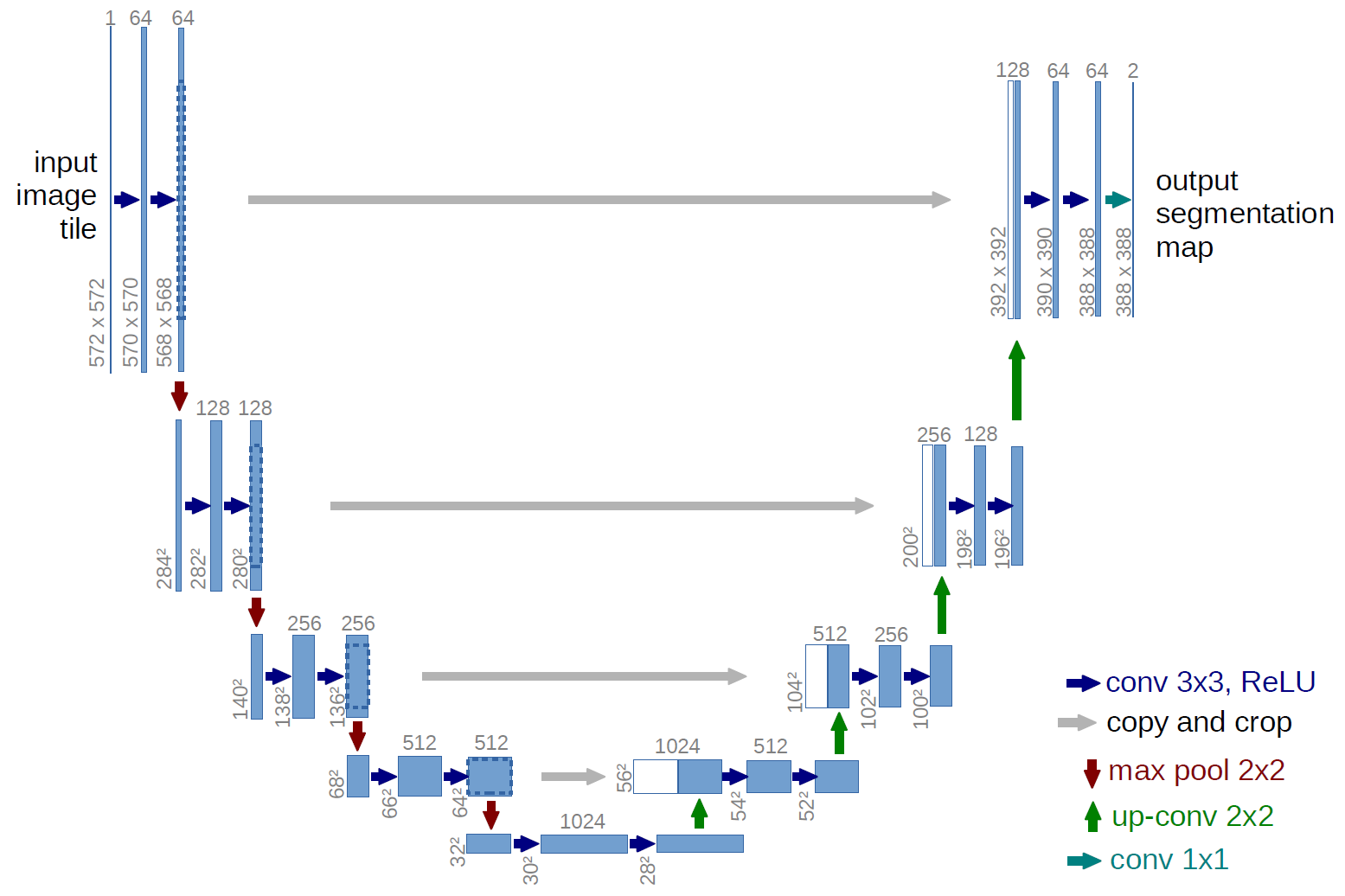
UNET, introduced by Ronneberger et al. in 2015, is a convolutional neural network designed specifically for biomedical image segmentation. Many state-of-the-art segmentation models still build on this architecture. It has several advantages over the sliding window approach:
It considers the full image context
It’s more efficient, requiring fewer training samples
It can handle varying sizes of target structures
In this lab, you’ll gain hands-on experience implementing the original UNET architecture, understanding its components, and applying it to medical imaging data.
Go to the utils/unet.py file and follow the instructions to implement the UNET architecture there. Run the cell below to test your implementation
[ ]:
from utils.unet import UNET
x = torch.randn((3, 1, 161, 161))
model = UNET(in_channels=1, out_channels=1)
preds = model(x)
assert preds.shape == x.shape, f"The output shape is not as expected got: {preds.shape} expected: {x.shape}"
print("UNET output shape is correct")
Now let’s train the model. We will be using the training data to train the model.
[ ]:
from utils.train import train

model = UNET(in_channels=1, out_channels=3)
loss_fn = torch.nn.CrossEntropyLoss()
optimizer = torch.optim.Adam(model.parameters(), lr=1e-3)
device = torch.device("cuda") if torch.cuda.is_available() else torch.device("cpu")
print(f"Using device: {device}")

trained_model = train(model, train_loader, loss_fn, optimizer, device=device, epochs=10)
# Save the model
torch.save(trained_model.state_dict(), 'trained_unet.pth')
[ ]:
# Plot results
# Function to plot segmentation results
def plot_segmentation_results(model, data_loader, num_samples=4):
    model.eval()
    with torch.no_grad():
        for batch in data_loader:
            images = batch['image'].to(device)
            labels = batch['label'].to(device)

            outputs = model(images)
            _, preds = torch.max(outputs, dim=1)

            images = images.cpu().numpy()
            labels = labels.cpu().numpy()
            preds = preds.cpu().numpy()

            fig, axes = plt.subplots(3, num_samples, figsize=(20, 12))
            for i in range(num_samples):
                axes[0, i].imshow(images[20+i, 0, :, :], cmap='gray')
                axes[0, i].set_title(f'Image {i+1}')
                axes[0, i].axis('off')

                axes[1, i].imshow(labels[20+i, 0, :, :], cmap='viridis')
                axes[1, i].set_title(f'True Label {i+1}')
                axes[1, i].axis('off')

                axes[2, i].imshow(preds[20+i, :, :], cmap='viridis')
                axes[2, i].set_title(f'Prediction {i+1}')
                axes[2, i].axis('off')

            plt.tight_layout()
            plt.show()
            break

# Plot results for training data
print("Training Data Results:")
plot_segmentation_results(trained_model, train_loader)

# Plot results for validation data
print("Validation Data Results:")
plot_segmentation_results(trained_model, val_loader)
Evaluating Segmentation Models: Beyond Accuracy#
We can hopefully see that the model is doing something that looks like it’s segmenting the image even though it is far from perfect. The question is; however, how can we quantify it? While accuracy is a common metric in classification tasks, it’s often inadequate for segmentation problems. Here’s why:
Class Imbalance: In many segmentation tasks, the region of interest (e.g., a tumor) may occupy only a small portion of the image. A model that simply predicts “background” for every pixel could achieve high accuracy but fail to segment the target region.
Spatial Information: Accuracy doesn’t account for the spatial relationship between predicted and true segmentations. It treats each pixel independently, missing important context.
Boundary Precision: Accuracy doesn’t differentiate between minor and major segmentation errors, which can be crucial in medical applications.
Better Alternatives#
Intersection over Union (IoU) / Jaccard Index:
Measures overlap between predicted and ground truth segmentations.
Range: 0 to 1 (higher is better).
Handles class imbalance well.
Dice Coefficient:
Similar to IoU but gives more weight to true positives.
Range: 0 to 1 (higher is better).
Widely used in medical image segmentation.
Mean IoU (mIoU):
Average IoU across all classes.
Useful for multi-class segmentation.
Hausdorff Distance:
Measures the maximum distance between predicted and true segmentation boundaries.
Important for assessing boundary accuracy.
These metrics provide a more comprehensive evaluation of segmentation performance, capturing aspects like overlap, boundary precision, and class balance that accuracy alone misses. Let’s first looks at what happens when we use accuracy as a metric.
[ ]:
def calculate_accuracy(model, data_loader, device):
    model.eval()
    correct = 0
    total = 0
    with torch.no_grad():
        for batch in data_loader:
            images = batch['image'].to(device)
            labels = batch['label'].to(device)

            outputs = model(images)
            _, preds = torch.max(outputs, dim=1)

            correct += (preds == labels.squeeze(1)).sum().item()
            total += labels.numel()

    return correct / total

# Calculate accuracy for the trained model
model_accuracy = calculate_accuracy(trained_model, val_loader, device)

# Calculate accuracy for predicting 0 everywhere
def zero_prediction_accuracy(data_loader, device):
    correct = 0
    total = 0
    for batch in data_loader:
        labels = batch['label'].to(device)
        correct += (labels == 0).sum().item()
        total += labels.numel()
    return correct / total

zero_pred_accuracy = zero_prediction_accuracy(val_loader, device)

print(f"Trained model accuracy: {model_accuracy*100:.2f}%")
print(f"Zero prediction accuracy: {zero_pred_accuracy*100:.2f}%")
As we can see the accuracy is not a good metric to evaluate the performance of the model since a model that predicts the same thing everywhere will have a high accuracy and our trained model does only perform slightly better than this. Let’s compute the mean IoU metric instead.
[ ]:
def calculate_iou(pred, target, num_classes, smooth=1e-6):
    ious = []
    for cls in range(num_classes):
        pred_cls = (pred == cls).float()
        target_cls = (target == cls).float()
        intersection = (pred_cls * target_cls).sum((1, 2))
        union = pred_cls.sum((1, 2)) + target_cls.sum((1, 2)) - intersection
        iou = (intersection + smooth) / (union + smooth)
        ious.append(iou.mean())
    return sum(ious) / len(ious)

def calculate_model_iou(model, data_loader, device, num_classes):
    model.eval()
    total_iou = 0
    num_batches = 0
    with torch.no_grad():
        for batch in data_loader:
            images = batch['image'].to(device)
            labels = batch['label'].to(device)

            outputs = model(images)
            preds = outputs.argmax(dim=1)

            iou = calculate_iou(preds, labels.squeeze(1), num_classes)
            total_iou += iou.item()
            num_batches += 1

    return total_iou / num_batches

def calculate_zero_pred_iou(data_loader, device, num_classes):
    total_iou = 0
    num_batches = 0
    for batch in data_loader:
        labels = batch['label'].to(device)
        zero_pred = torch.zeros_like(labels.squeeze(1))
        iou = calculate_iou(zero_pred, labels.squeeze(1), num_classes)
        total_iou += iou.item()
        num_batches += 1
    return total_iou / num_batches

# Assuming 3 classes (background + 2 hippocampus regions)
num_classes = 3

# Calculate IoU for the trained model
model_iou = calculate_model_iou(trained_model, val_loader, device, num_classes)

# Calculate IoU for zero prediction
zero_pred_iou = calculate_zero_pred_iou(val_loader, device, num_classes)

train_iou = calculate_model_iou(trained_model, train_loader, device, num_classes)
print(f"Trained model mean IoU: {model_iou:.4f}")
print(f"Zero prediction mean IoU: {zero_pred_iou:.4f}")
print(f"Trained model mean IoU on training set: {train_iou:.4f}")
If your UNET implementation is correct you should see that the IoU metric (> 0.85) is much better at quantifying the performance of the model compared to accuracy. In this case we include the background class in the calculation, but often it is excluded, that is essentially 66 % of the pixels are ignored in the calculation. In this case mean iou for the zero prediction would be 0.
Dice Coefficient for Image Segmentation#
The Dice coefficient is a widely used metric to evaluate the performance of image segmentation models. In the context of segmentation, it measures the overlap between the predicted segmentation mask and the ground truth mask. The Dice coefficient is defined as:
Where: - \(X\) is the set of pixels in the predicted segmentation mask - \(Y\) is the set of pixels in the ground truth mask - \(|X \cap Y|\) represents the number of pixels that are correctly segmented (true positives) - \(|X|\) and \(|Y|\) are the total number of pixels in the predicted and ground truth masks, respectively
In practical terms: - A Dice score of 1 indicates perfect overlap (ideal segmentation) - A Dice score of 0 indicates no overlap (worst-case segmentation)
The Dice coefficient is particularly useful in medical image segmentation because: 1. It’s sensitive to both over-segmentation and under-segmentation 2. It handles class imbalance well, which is common in medical images where the region of interest may be small compared to the background 3. It provides a single, interpretable value to assess segmentation quality
When calculating the Dice coefficient for multi-class segmentation, it’s often computed separately for each class and then averaged to get an overall score. We also average over the entire dataset to get a single score. Please complete the DiceScore class in the utils/metrics.py file.
[ ]:
from utils.metrics import DiceScore

# Initialize DiceScore
dice_metric = DiceScore()

# Function to calculate Dice score for the model
def calculate_dice_score(model, data_loader, device):
    model.eval()
    dice_metric.reset()
    with torch.no_grad():
        for batch in data_loader:
            images = batch['image'].to(device)
            labels = batch['label'].to(device)

            outputs = model(images)

            # Calculate Dice score for this batch
            batch_dice = dice_metric.calculate(labels.squeeze(1), outputs)

    # Compute the final mean Dice score
    return dice_metric.mean()

# Calculate Dice score for the trained model
model_dice = calculate_dice_score(trained_model, val_loader, device)

print(f"Trained model Dice score on Validation set: {model_dice:.4f}")
# Training set dice score
model_dice = calculate_dice_score(trained_model, train_loader, device)
print(f"Trained model Dice score on Training set: {model_dice:.4f}")
Question#
From these results, we can see the model is performing similarly on the training and validation set. What conclusions can you draw from this?